#Epidemic Analysis

#Preset Dynamics

The SIRSD Epidemic preset has $4$ cell states: Dead, Susceptible, Infectious, and Recovered. Its ordered rules are:

Infection probability saturates at $1$ Infectious neighbor: having $2$ through $8$ Infectious neighbors does not increase the $50\%$ roll. Because rules are evaluated in order, the death roll is attempted only after the recovery roll fails. Given that rolls are independent, that makes the unconditional $1$-generation death probability approximately $0.95\cdot0.1\%=0.095\%$ for an Infectious cell.

Recovered cells can become Susceptible again, so reinfection and multiple waves are possible. Dead cells remain Dead. There are no births, movement, or incubation state.

#Derived Metrics

Initial population, written as $N_0$, is the first recorded Susceptible + Infectious + Recovered count. Empty grid cells are not included.

• Prevalence: current Infectious cells divided by fixed $N_0$.
• Peak prevalence: maximum unsmoothed prevalence during the run.
• Mortality fraction: deaths occurring during the run divided by $N_0$.
• Final healthy grid density: final $\frac{\texttt{Susceptible}+\texttt{Recovered}}{512^2}$. This uses the whole grid as its denominator.
• Infectious duration: final Infectious generation minus first recorded generation.
• Time to peak: peak-Infectious generation minus first recorded generation.

Using fixed $N_0$ for prevalence prevents deaths from shrinking the denominator and artificially inflating late prevalence.

#Infection Episodes

An infection episode is $1$ reconstructed Susceptible → Infectious transition. The initial $12$ seeded Infectious cells are not counted.
With the preset's only $4$ possible transitions, the population deltas and changed_cells identify the aggregate flows exactly for consecutive generations.

If $C$ is changed_cells, the reconstruction is:

Episodes per initial population are cumulative $\frac{S\rightarrow I}{N_0}$. Values can exceed $1$ because the same population can pass through $R \rightarrow S \rightarrow I$ repeatedly. This is an event rate over the initial population, not the fraction of unique people ever infected and not a distribution of infections per individual.

#Density Outcomes

The clearest observed change is between $41\%$ and $42\%$: median episodes per initial population increase from $0.0717$ to $1.8876$, peak prevalence from $0.403\%$ to $3.211\%$, mortality from $0.135\%$ to $3.519\%$, and duration from $1\,092$ to $3\,189.5$ generations.

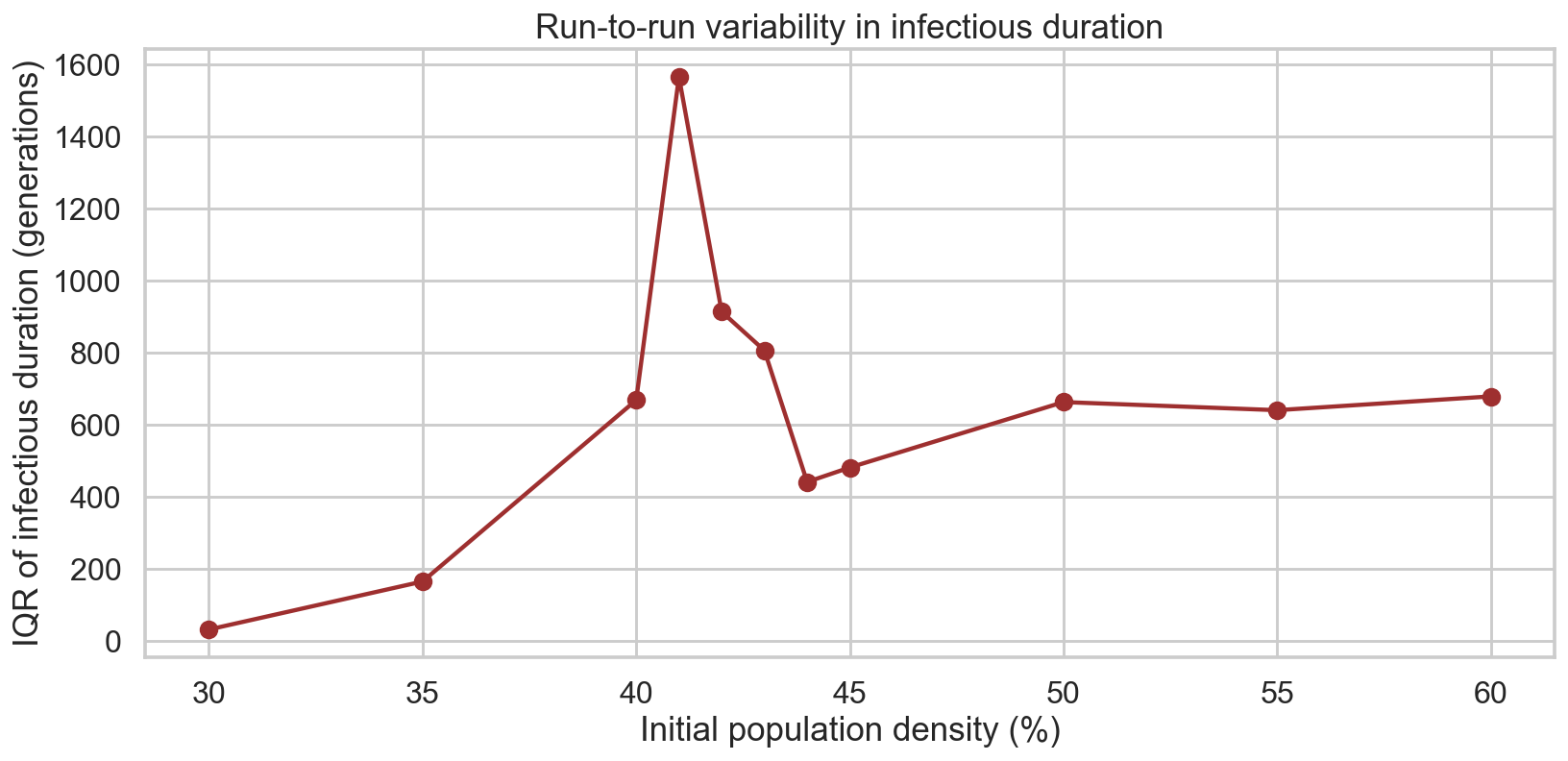
Run-to-run variation in infectious duration is greatest at $41\%$: its IQR is $1\,566.25$ generations, compared with $669.25$ at $40\%$ and $914.5$ at $42\%$.

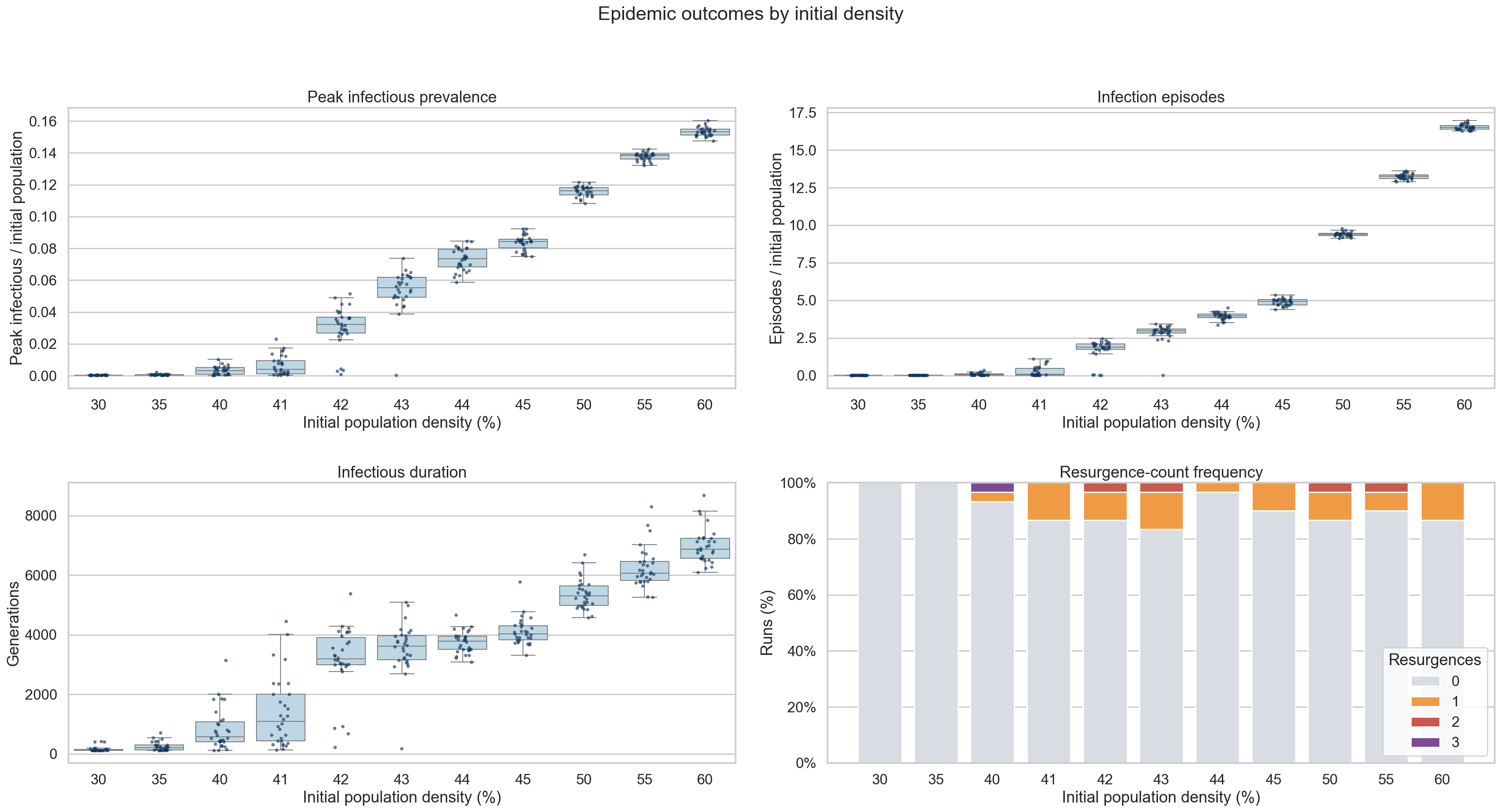
Resurgence count is explained below.

#Mortality And Surviving Population

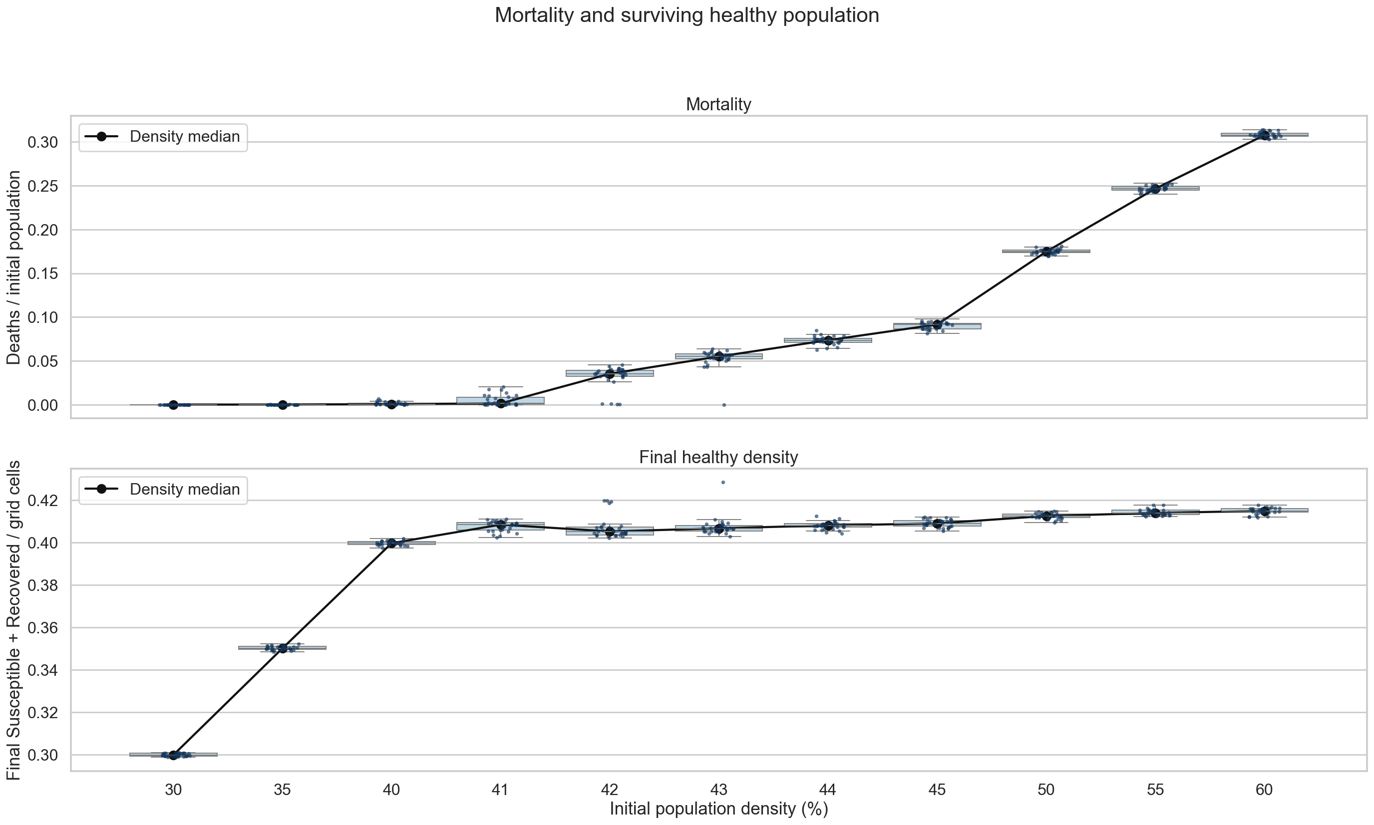
Above the transition, increased initial density supports many cycles of infection and substantially higher mortality. Median mortality reaches $30.783\%$ of the initial population at $60\%$ density.

Median final healthy grid density nevertheless stays in a narrow band from $40.521\%$ at $42\%$ to $41.493\%$ at $60\%$. This convergence is consistent with the regime transition observed between $41\%$ and $42\%$: at initial densities of $40\%$ or below, infection usually becomes extinct before spreading through enough of the population to cause substantial mortality, so final healthy density remains close to initial density. Above the transition, infection reaches a much larger part of the population and deaths progressively reduce occupancy. The epidemic therefore appears to prune densely populated grids toward a density at which continued transmission becomes difficult.

#Timing And Trajectories

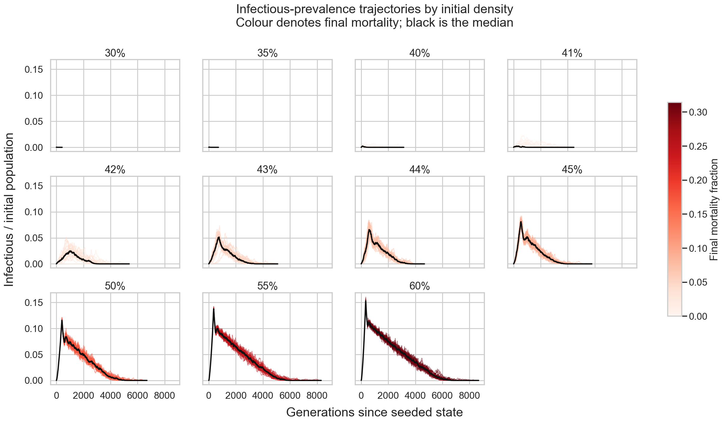
Median duration increases throughout the sustained-epidemic regime, reaching $6\,877.5$ generations at $60\%$. Time to peak behaves differently: it is largest at $42\%$ with a median of $1\,010$ generations, then falls to $733$ at $43\%$, $535.5$ at $45\%$, $409$ at $50\%$, and $334$ at $60\%$. Once dense local connectivity supports sustained spread, higher density produces an earlier, larger peak but a longer period of repeated circulation.

The spaghetti plots show all $30$ prevalence trajectories per density. Color denotes final mortality and the black curve is the per-generation median.

#Resurgence Count

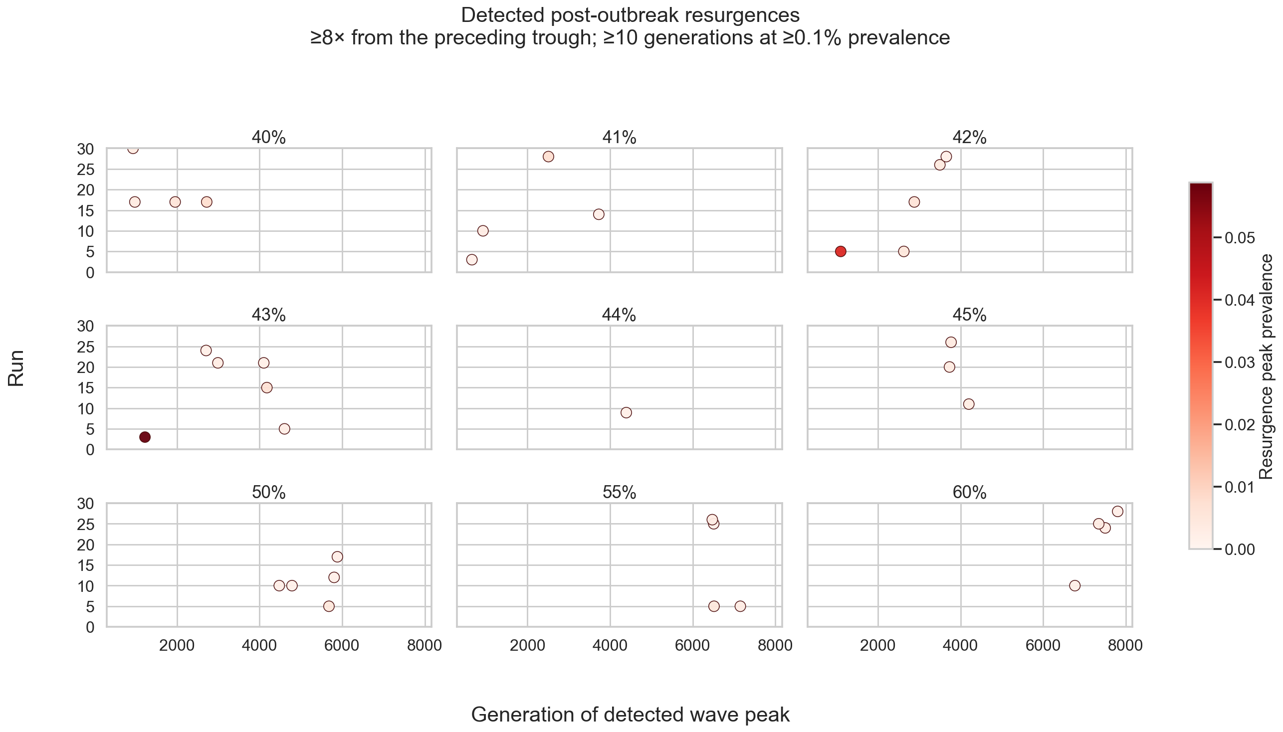
Resurgence is a retrospective event definition applied to prevalence, not a native engine metric.

1. Smooth prevalence with an $11$-generation centered mean. The window suppresses short cell-level fluctuations while keeping $5$ generations of context on either side.
2. Start a candidate wave when smoothed prevalence reaches $0.15\%$.
3. End it after smoothed prevalence remains at or below $0.05\%$ for $25$ consecutive generations.
4. Treat the first candidate as the initial outbreak.
5. Count a later candidate as a resurgence only if its smoothed peak is at least $8$ times the preceding smoothed trough, it spends at least $10$ generations at or above $0.15\%$, and the trough is above $0$.

The event's reported peak prevalence is the unsmoothed maximum inside its interval. Because the smoother is centered, this is an offline detector that uses future and past values; it is not suitable for real-time alerts.

Across all $330$ runs:

• $300$ runs have no resurgence.
• $25$ have $1$.
• $4$ have $2$.
• $1$ has $3$.
• $30$ runs, or $9.09\%$, have at least $1$, for $36$ qualifying resurgence events in total.
• No qualifying resurgence occurs at $30\%$ or $35\%$.

Counts are sparse and non-monotonic, so they support occasional post-outbreak resurgence but not a density-dependent resurgence law.

#Three-Resurgence Example

At $40\%$ density, run $17$ contains $3$ qualifying resurgences after its initial outbreak. In the recording, rendered at $30\text{ generations/s}$, the first occurs at generation $660$ ($\sim00{:}22$), the second at generation $1\,700$ ($\sim00{:}57$), and the third at generation $2\,400$ ($\sim01{:}20$). They subsequently peak at generations $980$ ($\sim00{:}32$), $1\,956$ ($\sim01{:}05$), and $2\,720$ ($\sim01{:}30$), with unsmoothed peak prevalences of approximately $0.345\%$, $0.567\%$, and $0.776\%$, respectively.
The recording provides a concrete example of the retrospective event definition above.

#Representative Runs

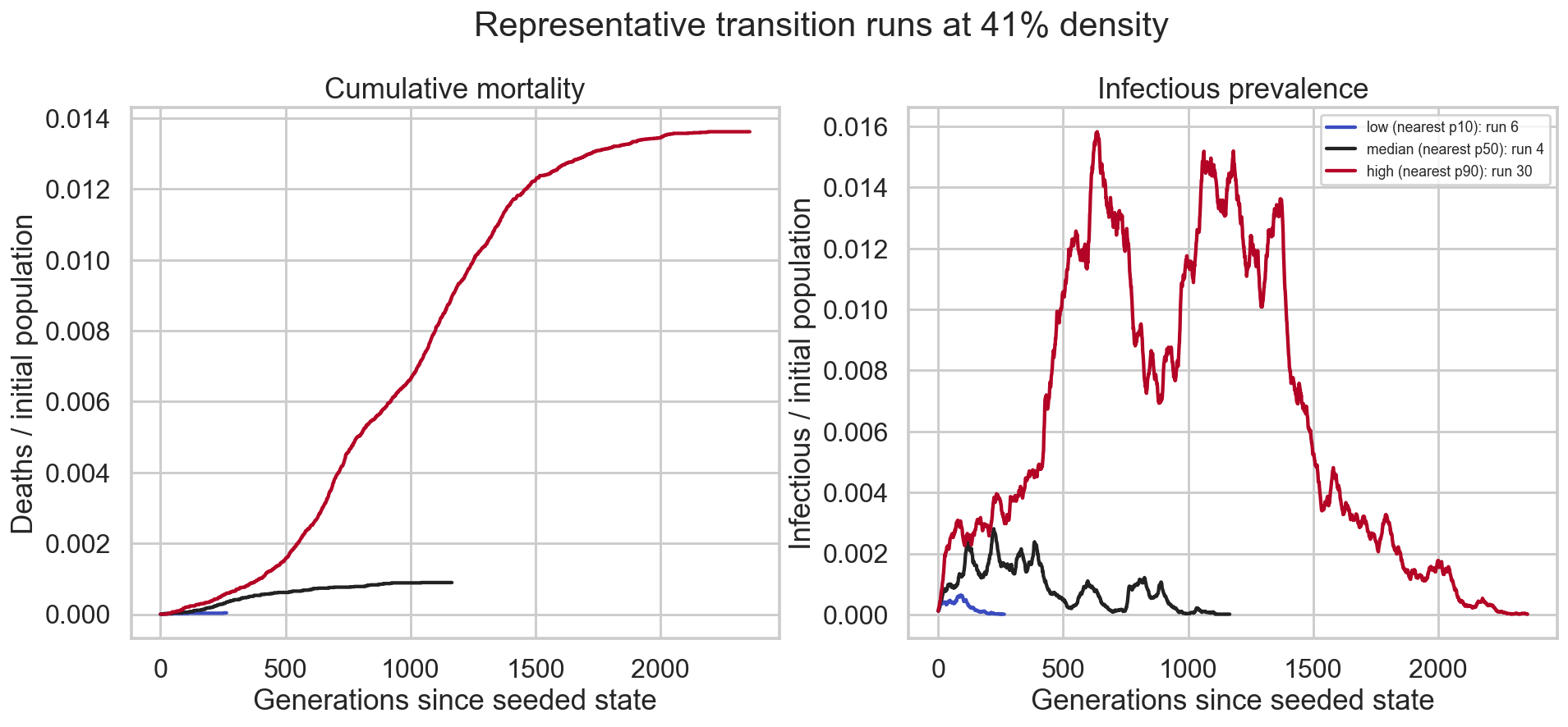
The transition figure uses $41\%$, where the infection-episode IQR is largest, and selects actual runs nearest the $10\text{th}$, $50\text{th}$, and $90\text{th}$ episode percentiles:

#Transition Runs In Motion

These recordings use the same $41\%$ initial density and correspond to the low-, median-, and high-outcome representatives above. They expose the run-to-run variation hidden by a density-level median.

#Typical Runs Across Regimes

The following median-like runs contrast rapid extinction at $30\%$ with sustained circulation and extensive mortality at $60\%$. To keep the long $60\%$ recording practical to view, it is rendered at $120\text{ generations/s}$, or $4\times$ the $30\text{ generations/s}$ used for the other videos. Its accelerated playback is a presentation choice made to reduce size and length and should not be used to compare visual propagation speed directly with other recordings.